# @hidden_cell
# The project token is an authorization token that is used to access project resources like data sources, connections, and used by platform APIs.
from project_lib import Project
project = Project(project_id='...', project_access_token='...')

Load and Visualize IBM Debater® Sentiment Composition Lexicons

In this notebook you will load, explore, clean and visualize data from the IBM Debater Sentiment Composition Lexicons dataset. The dataset includes sentiment composition lexicons and sentiment lexicons:

1. Sentiment composition lexicons containing 2,783 words.
2. Sentiment lexicons containing 66,058 unigrams and 262,555 bigrams.

The dataset addresses sentiment composition – predicting the sentiment of a phrase from the interaction between its constituents. For example, in the phrases “reduced bureaucracy” and “fresh injury”, both “reduced” and “fresh” are followed by a negative word. However, “reduced” flips the negative polarity, resulting in a positive phrase, while “fresh” propagates the negative polarity to the phrase level, resulting in a negative phrase. Accordingly, “reduced” is part of our “reversers” lexicon, and “fresh” is part of the “propagators” lexicon.

The dataset can be obtained for free from IBM Developer Data Asset Exchange.

Table of Contents

• 0. Prerequisite
• 1. Load Data
  • 1.1 About
  • 1.2 Read Data
• 2. Data Visualization
  • 2.1 Unigram
  • 2.2 Bigram
• 3. Save the Cleaned Data
• Authors

0. Prerequisites

Before you run this notebook complete the following steps:

• Insert a project token
• Import required modules

Insert a project token

When you import this project from the Watson Studio Gallery, a token should be automatically generated and inserted at the top of this notebook as a code cell such as the one below:

# @hidden_cell
# The project token is an authorization token that is used to access project resources like data sources, connections, and used by platform APIs.
from project_lib import Project
project = Project(project_id='YOUR_PROJECT_ID', project_access_token='YOUR_PROJECT_TOKEN')
pc = project.project_context

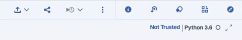
If you do not see the cell above, follow these steps to enable the notebook to access the dataset from the project's resources:

• Click on More -> Insert project token in the top-right menu section

• This should insert a cell at the top of this notebook similar to the example given above.

  If an error is displayed indicating that no project token is defined, follow these instructions.

• Run the newly inserted cell before proceeding with the notebook execution below

Import required modules

Import and configure the required modules.

# Define required imports
import pandas as pd
from pandas import read_excel
import numpy as np
import matplotlib.pyplot as plt
import plotly.graph_objs as go
import seaborn as sns
!pip install cufflinks
import cufflinks as cf
cf.go_offline()
cf.set_config_file(offline=False, world_readable=True)
from sklearn.feature_extraction.text import CountVectorizer
from IPython.display import clear_output
clear_output()

1. Load Data

1.1 About

The goal of this set of notebooks is to use the IBM Debater Sentiment Composition Lexicons dataset to categorize text on a sentence level, or as a whole, with a range of sentiments. This could be used in an application which collects customer feedback to help determine customer satisfaction.

Let's first explain a few definitions:

• Sentiment Analysis: Using natural language processing to determine the sentiment of a piece of text, e.g. determine if the text has a positive, negative, or neutral connotation.

• N-gram: a sequence of N terms

• Unigram: an N-gram with one term, e.g. “hello”

• Bi-gram: an N-gram with two terms, e.g. “hello world”

• POS (part of speech) tag: a word's part of speech, e.g. the POS tag for "dog" would be noun (or NN in the NLTK Python library).

1.2 Read Data

The first step is to load, and then modify the LEXICON_UG.txt and LEXICON_BG.txt datasets to include a sentiment column that is based on the SENTIMENT_SCORE column, but uses 1 or 0, where 1 is positive sentiment and 0 is negative sentiment.

# Define get data file function
def get_file_handle(fname):
    # Project data path for the raw data file
    data_path = project.get_file(fname)
    data_path.seek(0)
    return data_path

LEXICON_UG.txt:

This is a list of 66,058 unigrams and their predicted sentiment score. Note that in the paper Learning Sentiment Composition from Sentiment Lexicons, for unigrams that have sentiment in the HL lexicon (the publicly-available sentiment lexicon of Hu and Liu (2004)), the original sentiment from the HL lexicon (+1 or -1) was used, and not the predicted score. This step is not reflected in the released lexicon.

# define filename
DATA_PATH = 'LEXICON_UG.txt'

# Using pandas to read the data 
data_path = get_file_handle(DATA_PATH)
unigrams = pd.read_csv(data_path, sep=" ")
unigrams.head()

	UNIGRAM	SENTIMENT_SCORE
0	aa	0.019674
1	aaa	0.032775
2	aaas	0.074593
3	aachen	0.011926
4	aah	0.118070

LEXICON_BG.txt:

This is a list of 262,555 selected bigrams in the following format:

• Column 1: the bigram
• Column 2: the OpenNLP POS tags of its unigrams
• Column 3: the predicted sentiment score

# define filename
DATA_PATH = 'LEXICON_BG.txt'

# Using pandas to read the data 
data_path = get_file_handle(DATA_PATH)
bigrams = pd.read_csv(data_path, sep=" ")
bigrams.head()

	BIGRAM	POS_TAGS	SENTIMENT_SCORE
0	abalone-divers	NN-NNS	-0.090230
1	abandoned-animals	VBN-NNS	-0.089895
2	abandoned-apartment	VBN-NN	-0.126907
3	abandoned-attempts	VBN-NNS	-0.053709
4	abandoned-babies	VBN-NNS	-0.074742

2. Data Visualization

In this section, we will visualize the unigrams and bigrams datasets.

2.1 Unigrams

First, let's categorize the sentiment of each term.

# Add sentiment column
unigrams['sentiment'] = np.where(unigrams['SENTIMENT_SCORE'] > 0, 1, 0)  # 1 is positive, 0 is negative
unigrams.head()

	UNIGRAM	SENTIMENT_SCORE	sentiment
0	aa	0.019674	1
1	aaa	0.032775	1
2	aaas	0.074593	1
3	aachen	0.011926	1
4	aah	0.118070	1

We want to check the distribution of the review sentiment polarity score.

# The distribution of review sentiment polarity score
unigrams['SENTIMENT_SCORE'].iplot(
    kind='hist',
    bins=50,
    xTitle='polarity',
    linecolor='black',
    yTitle='count',
    title='Sentiment Polarity Distribution')
# The sentiment polarity score is similar to a bell curve, center at 0, means half of them are positive, half are negative.

The distribution of sentiment polarity is a bell-shaped curve.

Then, let's check the unigram text length distribution.

# Get the string length of each unigram word
unigrams['uni_len'] = [len(str(i)) for i in unigrams['UNIGRAM']]
# Plot the unigram length distribution
unigrams['uni_len'].iplot(
    kind='hist',
    xTitle='unigram length',
    linecolor='black',
    yTitle='count',
    title='Unigram Text Length Distribution')

The distribution of unigram text length is also approximately normally distributed, which means our dataset is balanced.

We are now saving the first letter of each term.

unigrams['first_letter'] = unigrams.UNIGRAM.str[0]
unigrams.head()

	UNIGRAM	SENTIMENT_SCORE	sentiment	uni_len	first_letter
0	aa	0.019674	1	2	a
1	aaa	0.032775	1	3	a
2	aaas	0.074593	1	4	a
3	aachen	0.011926	1	6	a
4	aah	0.118070	1	3	a

In these mext steps, we group by the first letter and sentiment score of each term, and then count amount of unigrams under each category.

# get number of words under each alphabet
group_data = unigrams.groupby(['first_letter', 'sentiment'])
group_data.count()

		UNIGRAM	SENTIMENT_SCORE	uni_len
first_letter	sentiment
a	0	2022	2022	2022
	1	2041	2041	2041
b	0	2569	2569	2569
	1	1409	1409	1409
c	0	3595	3595	3595
	1	2787	2787	2787
d	0	2645	2645	2645
	1	1261	1261	1261
e	0	1293	1293	1293
	1	1413	1413	1413
f	0	1637	1637	1637
	1	1062	1062	1062
g	0	1242	1242	1242
	1	973	973	973
h	0	1531	1531	1531
	1	995	995	995
i	0	1594	1594	1594
	1	1013	1013	1013
j	0	400	400	400
	1	230	230	230
k	0	435	435	435
	1	301	301	301
l	0	1280	1280	1280
	1	931	931	931
m	0	2205	2205	2205
	1	1493	1493	1493
n	0	810	810	810
	1	592	592	592
o	0	962	962	962
	1	628	628	628
p	0	3001	3001	3001
	1	2094	2094	2094
q	0	168	168	168
	1	130	130	130
r	0	2023	2023	2023
	1	1730	1730	1730
s	0	4768	4768	4768
	1	2714	2714	2714
t	0	2035	2035	2035
	1	1351	1351	1351
u	0	1121	1121	1121
	1	446	446	446
v	0	539	539	539
	1	471	471	471
w	0	1123	1123	1123
	1	552	552	552
x	0	28	28	28
	1	28	28	28
y	0	116	116	116
	1	91	91	91
z	0	117	117	117
	1	61	61	61

Now, we visualize the distribution of the unigram count of all letters.

plt.figure(figsize=(20,20))
sns.set(style="darkgrid")
ax = sns.countplot(x="first_letter", data=unigrams)

plt.title('Data Distribution')

for p in ax.patches:
        total_count = str(p.get_height())
        x=p.get_x() + p.get_width() - 0.75
        y=p.get_y() +p.get_height()
        ax.annotate(total_count, (x, y))

In the unigrams dataset, the first letter normally starts with s or c while the least frequent letters are x, y, and z.

2.2 Bigrams

Similarly, we categorize the sentiment of each term, positive or negative.

# Add sentiment column
bigrams['sentiment'] = np.where(bigrams['SENTIMENT_SCORE'] > 0, 1, 0)  # 1 is positive, 0 is negative
bigrams.head()

	BIGRAM	POS_TAGS	SENTIMENT_SCORE	sentiment
0	abalone-divers	NN-NNS	-0.090230	0
1	abandoned-animals	VBN-NNS	-0.089895	0
2	abandoned-apartment	VBN-NN	-0.126907	0
3	abandoned-attempts	VBN-NNS	-0.053709	0
4	abandoned-babies	VBN-NNS	-0.074742	0

And then we visualize the sentiment polarity distribution.

# The distribution of review sentiment polarity score
bigrams['SENTIMENT_SCORE'].iplot(
    kind='hist',
    bins=50,
    xTitle='polarity',
    linecolor='black',
    yTitle='count',
    title='Sentiment Polarity Distribution')

We group by the POS-TAGS and sentiment score of each bigram term.

df = pd.DataFrame(bigrams.groupby(['POS_TAGS', 'sentiment']).size().reset_index())
df.head()

	POS_TAGS	sentiment	0
0	JJ-JJ	0	1698
1	JJ-JJ	1	2000
2	JJ-JJR	0	5
3	JJ-JJR	1	3
4	JJ-JJS	0	9

Visualize the histograms of pos-tags and show the count of positive versus negative sentiment.

import plotly.express as px

fig = px.bar(df, x="POS_TAGS", y=0, color="sentiment", title="Long-Form Input")
fig.show()

bigrams.groupby('POS_TAGS').count()['SENTIMENT_SCORE'].sort_values(ascending=False).iplot(kind='bar', yTitle='Count', linecolor='black', opacity=0.8,
                                                           title='Pos Tags Count', xTitle='Pos Tag')

# get number of words under each POS Tag
group_data = bigrams.groupby(['POS_TAGS','sentiment'])
group_data.count()

		BIGRAM	SENTIMENT_SCORE
POS_TAGS	sentiment
JJ-JJ	0	1698	1698
	1	2000	2000
JJ-JJR	0	5	5
	1	3	3
JJ-JJS	0	9	9
...	...	...	...
VBP-NNS	1	151	151
VBZ-NN	0	326	326
	1	609	609
VBZ-NNS	0	179	179
	1	743	743

91 rows × 2 columns

# add first letter and sentiment columns
bigrams['first_letter'] = bigrams.BIGRAM.str[0]
# get number of words under each alphabet
group_data = bigrams.groupby(['first_letter','sentiment'])
group_data.count()

		BIGRAM	POS_TAGS	SENTIMENT_SCORE
first_letter	sentiment
a	0	6784	6784	6784
	1	7192	7192	7192
b	0	7012	7012	7012
	1	5127	5127	5127
c	0	12077	12077	12077
	1	11856	11856	11856
d	0	9196	9196	9196
	1	6117	6117	6117
e	0	6377	6377	6377
	1	9498	9498	9498
f	0	7880	7880	7880
	1	5584	5584	5584
g	0	3486	3486	3486
	1	4278	4278	4278
h	0	4982	4982	4982
	1	3664	3664	3664
i	0	6628	6628	6628
	1	6920	6920	6920
j	0	673	673	673
	1	349	349	349
k	0	532	532	532
	1	486	486	486
l	0	5206	5206	5206
	1	4531	4531	4531
m	0	7747	7747	7747
	1	6936	6936	6936
n	0	2711	2711	2711
	1	2348	2348	2348
o	0	3872	3872	3872
	1	3459	3459	3459
p	0	11531	11531	11531
	1	9215	9215	9215
q	0	486	486	486
	1	654	654	654
r	0	7508	7508	7508
	1	7032	7032	7032
s	0	16508	16508	16508
	1	13062	13062	13062
t	0	6951	6951	6951
	1	5667	5667	5667
u	0	5066	5066	5066
	1	2353	2353	2353
v	0	2427	2427	2427
	1	2606	2606	2606
w	0	4293	4293	4293
	1	2677	2677	2677
x	0	7	7	7
	1	6	6	6
y	0	268	268	268
	1	620	620	620
z	0	87	87	87
	1	23	23	23

plt.figure(figsize=(20,20))
sns.set(style="darkgrid")
ax = sns.countplot(x="first_letter", data=bigrams)

plt.title('Data Distribution')

for p in ax.patches:
        total_count = str(p.get_height())
        x=p.get_x() + p.get_width() - 0.75
        y=p.get_y() +p.get_height()
        ax.annotate(total_count, (x, y))

3. Save the Cleaned Data

Finally, we save the cleaned dataset as a Project asset for later re-use. You should see similar to the following after saving the file:

{'file_name': 'bigrams.csv',
 'message': 'File saved to project storage.',
 'bucket_name': 'ibmdebatersentimentcompositionlex-...',
 'asset_id': '...'}

Note: In order for this step to work, your project token (see the first cell of this notebook) must have Editor role. By default this will overwrite any existing file.

project.save_data("unigrams.csv", unigrams.to_csv(float_format='%g'), overwrite=True)
project.save_data("bigrams.csv", bigrams.to_csv(float_format='%g'), overwrite=True)

Next steps

• Close this notebook.
• Open the Part 2 - Model Development notebook to explore the cleaned dataset.

Citation

Toledo-Ronen et. al, Learning Sentiment Composition from Sentiment Lexicons, COLING 2018

Authors

This notebook was created by the Center for Open-Source Data & AI Technologies.

---

Copyright © 2021 IBM. This notebook and its source code are released under the terms of the MIT License.